Table of Contents
What is COUNTIFS in Excel?
The COUNTIFS excel function counts the values of the supplied range based on one or multiple criteria (conditions). The supplied range can be single or multiple and adjacent or non-adjacent. Being a statistical function of Excel, the COUNTIFS supports the usage of comparison operators and wildcard characters.
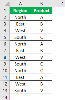
For example, given the following table, the COUNTIFS excel function can count the total number of products with the name “B” for the east region. The formula “=COUNTIFS(A2:A13,“EAST”,B2:B13,“B”)” returns 2.

The COUNTIFS is different from the COUNTIF function in the sense that the latter counts the values in a single range based on one condition.

You are free to use this image on your website, templates etc, Please provide us with an attribution linkHow to Provide Attribution?Article Link to be Hyperlinked
For eg:
Source: COUNTIFS Function in Excel (wallstreetmojo.com)
The Syntax of the COUNTIFS Excel Function
The syntax of the function is shown in the following image.

The function accepts the following arguments:
- Criteria_range1: This is the first range within which values are to be counted.
- Criteria1: This is the criteria (conditions) to be applied to “criteria_range1.” In other words, “criteria1” specifies the kind of cells which will be counted from “criteria_range1.”
- Criteria_range2: This is the second range within which values are to be counted.
- Criteria2: This is the criteria to be applied to “criteria_range2.” In other words, “criteria2” specifies the kind of cells which will be counted from “criteria_range2.”
The “criteria_range1” and “criteria1” are required arguments. The remaining range and criteria pairs are optional. In the COUNTIFs excel function, up to 127 range and criteria combinations can be specified.
Note 1: In case of multiple range and criteria pairs, the COUNTIFS counts only those cells that meet all the specified conditions.
Note 2: Every additional range should have the same number of rows and columns as the “criteria_range1.”
How to Use COUNTIFS Function in Excel?
Let us consider a few examples of COUNTIFS formula of Excel.
You can download this COUNTIFS Function Excel Template here – COUNTIFS Function Excel Template
Example #1–Two Conditions
The following table shows the region-wise products of an organization. The regions are categorized according to the four directions north, south, east, and west. The product names are displayed with a single letter.
We want to count the total number of products with the name “B” for the east region.
The steps to count cells with the help of the COUNTIFS excel function are listed as follows:
- Open the COUNTIFS formula.
- Select column A (region) as the “criteria_range1.” Alternatively, you can select column B (product).
- Select the “criteria1” for the range A2:A13. Since the cells matching the criterion “east” are to be counted, enter the same in the formula.
- Select column B (product) as the “criteria_range2.”
- Select the “criteria2” for the range B2:B13. Since the cells matching the criterion “B” are to be counted, enter the same in the formula.
- Press the “Enter” key. The output is 2, as shown in the succeeding image. This implies that for the east region, there are two products with the name “B.”
Hence, the output matches two conditions, region “east” and product “B.”
Though product “B” is also present in cell B12, it has been ignored by the COUNTIFS formula. This is because this cell corresponds to the west region.
Example #2–Three Conditions
Working on the data of example #1, we have added the names of the sales personnel (column C) to the dataset (shown in the succeeding image).
We want to count the total number of products “B” of the east region sold by Karan.

With the addition of a condition, we have to evaluate the data based on three criteria (region “east,” product “B,” and salesperson “Karan”).
In continuation with example #1 (preceding example), the additional steps are listed as follows:
Step 1: Enter the complete formula as written in example #1.
Step 2: Select column C (sales person) as the “criteria_range3.”
Step 3: Select the “criteria3” for the range C2:C13. Since the cells matching the criterion “Karan” are to be counted, enter the same in the formula.
Step 4: Press the “Enter” key. The output is 1, as shown in the succeeding image. This implies that for the east region, there is one product with the name “B” sold by the salesperson Karan.
Hence, the output matches three conditions, region “east,” product “B,” and salesperson “Karan.”
The total number of products corresponding to the name “B” and the region “east” is 2. However, with the addition of the criterion “Karan,” this count is reduced to 1.
Example #3–Comparison (Logical) Operators
The logical operatorsLogical OperatorsIn Excel, logical operators, also known as comparison operators, are used to compare two or more values. Depending on whether the condition matching is true or false, these operators return the output.read more are used in the COUTNIFS formula to structure the criteria. Let us consider an example of the same.
The following table shows the prices (in dollars) of the different products of an organization. The region in which each product is sold is also listed. The product names are displayed with a single letter.
We want to count the total number of products of the east region with the price greater than $20.

Step 1: Open the COUNTIFS formula.
Step 2: Select column C (region) as the “criteria_range1.”
Step 3: Select the “criteria1” for the range C2:C10. Since the cells matching the criterion “east” are to be counted, enter the same in the formula.
Step 4: Select column B (price) as the “criteria_range2.”
Step 5: Select the “criteria2” for the range B2:B10. Since the cells matching the criterion “>20” are to be counted, enter the same in the formula.
Note: The comparison operators in the “criteria” argument must be placed within double quotation marks.
Step 6: Press the “Enter” key. The output is 2, as shown in the following image. This implies that for the east region, there are two products with the price greater than $20.
Example #4–Date Values and Comparison Operators
The following table shows the dates and the amounts for which invoices are issued to the buyer.
We want to count the number of invoices sent (or issued) between 20-June-2019 to 26-June-2019.
The value between the two given dates (cell D2 and D3) has to be counted in column E, as shown by a question mark in the following image.
Step 1: Open the COUNTIFS excel function.
Step 2: Select column A (invoice date) as the “criteria_range1.”
Step 3: Since we need to count the invoices sent after 20-June-2019, enter the greater than symbol (>) within the double quotation marks.
Step 4: Enter the “criteria1” for the range A2:A10. The cell D2 contains the beginning issue date. Since the cells matching the criterion “>”&D2 are to be counted, enter the same in the formula.
The ampersand ($) is added before the cell reference D2. The cell D2 can be selected rather than typing manually.
Step 5: Select the “criteria_range2” which is the same as “criteria_range1,” i.e., A2:A10.
Step 6: Since we need to count the invoices sent before 26-June-2019, enter the less than symbol (<) within the double quotation marks. This is shown in the succeeding image.
Step 7: Enter the “criteria2” for the range A2:A10. The cell D3 contains the ending issue date. Since the cells matching the criterion “<”&D3 are to be counted, enter the same in the formula.
Step 8: Press the “Enter” key. The output is 3, as shown in the following image. This implies that three invoices are sent between the dates 20-June-2019 and 26-June-2019.
Frequently Asked Questions
Define the COUNTIFS function of Excel.
The COUNTIFS function counts cells of a given range based on one or multiple conditions (criteria). It counts only those cells which meet all the stated conditions. The syntax of the function is given as follows:
“=COUNTIFS(criteria_range1,criteria1,[criteria_range2,criteria2]…)”
The “criteria_range1” is the first range whose values are to be counted based on the fulfillment of “criteria1” (condition). The first range and criteria pair is required, while the remaining are optional.
How does the COUNTIFS function of Excel work with multiple criteria?
The COUNTIFS works with multiple criteria in the following way:
With multiple criteria (AND logic)
The usual COUNTIFS counts the cells that satisfy all the stated conditions. In other words, it counts those cells for which all the conditions evaluate to “true.” This is the AND logic and the formula is the same as the general syntax of the COUNTIFS function.
With multiple criteria (OR logic)
In this case, the COUNTIFS counts the cells for which at least one of the stated conditions evaluates to “true.” This is the OR logic and either of the following formulas can be used in this case:
• “=COUNTIFS(criteria_range1,criteria1,[criteria_range2,criteria2])+COUNTIFS(criteria_range1,criteria1,[criteria_range2,criteria2])”
• “=SUM(COUNTIFS(range,{“criteria1”,“criteria2”,“criteria3”,…}))”
Note: The COUNTIFS embed within the SUM function specifies all the criteria in an array constant.
How to use the COUNTIFS function of Excel with the operator “not equal to” (<>)?
The comparison operator “not equal to” (<>) counts the cells that are not equal to the given condition. For instance, the range A1:A8 consists of rose, lotus, daisy, sunflower, lily, marigold, rose, and lily.
The formula “=COUNTIFS(A1:A8,“<>rose”,A1:A8,“<>lotus”)” counts the cells in the range A1:A8, which are not equal to “rose” and “lotus.” Hence, the formula returns 5.
Recommended Articles
This has been a guide to COUNTIFS function in Excel. Here we discuss how to use the COUNTIFS excel formula along with practical examples and a downloadable Excel template. You may learn more about Excel from the following articles –
- 35+ Courses
- 120+ Hours
- Full Lifetime Access
- Certificate of Completion
LEARN MORE >>