Hyperlink in Excel: how to create, edit and remove

Bạn đang xem: Hyperlink in Excel: how to create, edit and remove

The tutorial explains how to hyperlink in Excel by using 3 different methods. You will learn how to insert, change and remove hyperlinks in your worksheets and now to fix non-working links.

Hyperlinks are widely used on the Internet to navigate between web-sites. In your Excel worksheets, you can easily create such links too. In addition, you can insert a hyperlink to go to another cell, sheet or workbook, to open a new Excel file or create an tin nhắn hộp thư online message. This tutorial provides the detailed guidance on how to do this in Excel 2016, 2013, 2010 and earlier versions.

What is hyperlink in Excel

An Excel hyperlink is a reference to a specific location, document or web-page that the user can jump to by clicking the link.

Microsoft Excel enables you to create hyperlinks for many different purposes including:

• Going to a certain location within the current workbook
• Opening another document or getting to a specific place in that document, e.g. a sheet in an Excel file or bookmark in a Word document.
• Navigating to a web-page on the Internet or Intranet
• Creating a new Excel file
• Sending an tin nhắn hộp thư online to a specified address

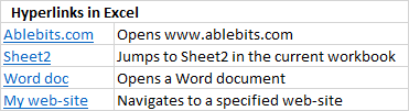
Hyperlinks in Excel are easily recognizable – generally this is text highlighted in underlined blue like shown in the screenshot below.

Absolute and relative hyperlinks in Excel

Microsoft Excel supports two types of links: absolute and relative, depending on whether you specify a full or partial address.

An absolute hyperlink contains a full address, including the protocol and tên miền name for URLs, and the entire path and file name for documents. For example:

Absolute URL: https://www.ablebits.com/excel-lookup-tables/index.php

Absolute link to an Excel file: C:Excel filesSource DataBook1.xlsx

A relative hyperlink contains a partial address. For example:

Relative URL: excel-lookup-tables/index.php

Relative link to an Excel file: Source dataBook3.xlsx

On the website, it’s a common practice to use relative URLs. In your Excel hyperlinks, you should always supply full URLs for web-pages. Though, Microsoft Excel can understand URLs without a protocol. For example, if you type “www.ablebits.com” in a cell, Excel will automatically add the default “http” protocol and convert it into a hyperlink you can follow.

When creating links to Excel files or other documents stored on your computer, you can use either absolute or relative addresses. In a relative hyperlink, a missing part of the file path is relative to the location of the active workbook. The main advantage of this approach is that you don’t have to edit the link address when the files are moved to another location. For example, if your active workbook and target workbook reside on drive C, and then you move them to drive D, relative hyperlinks will continue working as long as the relative path to the target file remains unchanged. In case of an absolute hyperlink, the path should be updated every time the file is moved to another place.

How to create a hyperlink in Excel

In Microsoft Excel, the same task can often be accomplished in a few different ways, and it is also true for creating hyperlinks. To insert a hyperlink in Excel, you can use any of the following:

The most common way to put a hyperlink directly into a cell is by using the Insert Hyperlink dialog, which can be accessed in 3 different ways. Just select the cell where you want to insert a link and do one of the following:

• On the Insert tab, in the Links group, click the Hyperlink
  
• Right click the cell, and select Hyperlink… from the context thực đơn.
  
• Press the

  Ctrl + K

  shortcut.

And now, depending on what sort of link you want to create, proceed with one of the following examples:

Create hyperlink to another document

To insert a hyperlink to another document such as a different Excel file, Word document or PowerPoint presentation, open the Insert Hyperlink dialog, and perform the steps below:

1. On the left-hand panel, under Link to, click the Existing File or Website Page
2. In the Look in list, browse to the location of the target file, and then select the file.
3. In the Text to display box, type the text you want to appear in the cell (“Book3” in this example).
4. Optionally, click the ScreenTip… button in the upper-right corner, and enter the text to be displayed when the user hovers the mouse over the hyperlink. In this example, it’s “Goto Book3 in My Documents”.
5. Click OK.

The hyperlink is inserted in the selected cell and looks exactly as you’ve configured it:

To link to a specific sheet or cell, click the Bookmark… button in the right-hand part of the Insert Hyperlink dialog box, select the sheet and type the target cell address in the Type in the cell reference box, and click OK.

To link to a named range, select it under Defined names like shown below:

Add a hyperlink to a website address (URL)

To create a link to a website page, open the Insert Hyperlink dialog, and proceed with the following steps:

1. Under Link to, select Existing File or Website Page.
2. Click the Browse the Website button, open the website page you want to link to, and switch back to Excel without closing your website browser.

Excel will insert the website site Address and Text to display for you automatically. You can change the text to display the way you want, enter a screen tip if needed, and click OK to add the hyperlink.

Alternatively, you can sao chép the website page URL before opening the Insert Hyperlink dialog, and then simply paste the URL in the Address box.

Hyperlink to a sheet or cell in the current workbook

To create a hyperlink to a specific sheet in the active workbook, click the Place in this Document icon. Under Cell Reference, select the target worksheet, and click OK.

To create an Excel hyperlink to cell, type the cell reference in the Type in the cell reference box.

To link to a named range, select it under the Defined Names node.

Insert a hyperlink to open a new Excel workbook

Besides linking to existing files, you can create a hyperlink to a new Excel file. Here’s how:

1. Under Link to, click the Create New Document icon.
2. In the Text to display box, type the link text to be displayed in the cell.
3. In the Name of new document box, enter the new workbook name.
4. Under Full path, test the location where the newly created file will be saved. If you want to change the default location, click the Change button.
5. Under When to edit, select the desired editing option.
6. Click OK.

A hyperlink to create an tin nhắn hộp thư online message

Apart from linking to various documents, the Excel Hyperlink feature allows you to send an tin nhắn hộp thư online message directly from your worksheet. To have it done, follow these steps:

1. Under Link to, select the E-mail Address icon.
2. In the E-mail address box, type the e-mail address of your recipient, or multiple addresses separated with semicolons.
3. Optionally, enter the message subject in the Subject box. Please keep in mind that some browsers and e-mail clients may not recognize the subject line.
4. In the Text to display box, type the desired link text.
5. Optionally, click the ScreenTip… button and enter the text you want (the screen tip will be displayed when you hover over the hyperlink with the mouse).
6. Click OK.

Tip. The fastest way to make a hyperlink to a specific e-mail address it to type the address directly in a cell. As soon as you hit the Enter key, Excel will automatically convert it into a clickable hyperlink.

If you are one of those Excel pros that employ formulas to tackle most of the tasks, you can use the HYPERLINK function, which is specially designed to inset hyperlinks in Excel. It is particularly useful when you intend to create, edit or remove multiple links at a time.

The syntax of the HYPERLINK function is as follows:

HYPERLINK(link_location, [friendly_name])

Where:

• Link_location is the path to the target document or web-page.
• Friendly_name is the link text to be displayed in a cell.

For example, to create a hyperlink titled “Source data” that opens Sheet2 in the workbook named “Source data” stored in the “Excel files” folder on drive D, use this formula:

=HYPERLINK("[D:Excel filesSource data.xlsx]Sheet2!A1", "Source data")

For the detailed explanation of the HYPERLINK function arguments and formula examples to create various types of links, please see How to use Hyperlink function in Excel.

How to insert hyperlink in Excel by using VBA

To automate the creation of hyperlink in your worksheets, you can use this simple VBA code:

	Public Sub AddHyperlink()
	
			Sheets("Sheet1").Hyperlinks.Add Anchor:=Sheets("Sheet1").Range("A1"), Address:="", SubAddress:="Sheet3!B5", TextToDisplay:="My hyperlink"
	
	End Sub
	

Where:

• Sheets – the name of a sheet on which the link should be inserted (Sheet 1 in this example).
• Range – a cell where the link should be inserted (A1 in this example).
• SubAddress – link destination, i.e. where the hyperlink should point to (Sheet3!B5 in this example).
• TextToDisplay -text to be displayed in a cell (“My hyperlink” in this example).

Given the above, our macro will insert a hyperlink titled “My hyperlink” in cell A1 on Sheet1 in the active workbook. Clicking the link will take you to cell B5 on Sheet3 in the same workbook.

If you have little experience with Excel macros, you may find the following instructions helpful: How to insert and run VBA code in Excel

If you created a hyperlink by using the Insert Hyperlink dialog, then use a similar dialog to change it. For this, right-click a cell holding the link, and select Edit Hyperlink… from the context thực đơn or press the Crtl+K shortcut or click the Hyperlink button on the ribbon.

Whichever you do, the Edit Hyperlink dialog box will show up. You make the desired changes to the link text or link location or both, and click OK.

To change a formula-driven hyperlink, select the cell containing the Hyperlink formula and modify the formula’s arguments. The following tip explains how to select a cell without navigating to the hyperlink location.

To change multiple Hyperlink formulas, use Excel’s Replace All feature as shown in this tip.

How to change a hyperlink appearance

By default, Excel hyperlinks have a traditional underlined blue formatting. To change the default appearance of a hyperlink text, perform the following steps:

1. Go to the Home tab, Styles group, and either:
   • Right-click Hyperlink, and then click Modify… to change the appearance of hyperlinks that have not been clicked yet.
   • Right-click Followed Hyperlink, and then click Modify… to change the formatting of hyperlinks that have been clicked.

   

2. In the Style dialog box that appears, click Format…
   
3. In the Format Cells dialog, switch to the Font and/or Fill tab, apply the options of your choosing, and click OK. For example, you can change the font style and font color like shown in the screenshot below:
   
4. The changes will be immediately reflected in the Style dialog. If upon a second thought, you decide not to apply certain modifications, clear the test boxes for those options.
   
5. Click OK to save the changes.

Note. All changes made to the hyperlink style will apply to all hyperlinks in the current workbook. It is not possible to modify formatting of individual hyperlinks.

Removing hyperlinks in Excel is a two-click process. You simply right-click a link, and select Remove Hyperlink from the context thực đơn.

This will remove a clickable hyperlink, but keep the link text in a cell. To delete the link text too, right-click the cell, and then click Clear Contents.

Tip. To remove all or selected hyperlinks at a time, use the Paste Special feature as demonstrated in

To remove all or selected hyperlinks at a time, use the Paste Special feature as demonstrated in How remove multiple hyperlinks in Excel

Now that you know how to create, change and remove hyperlinks in Excel, you may want to learn a couple of useful tips to work with links most efficiently.

How to select a cell containing a hyperlink

By default, clicking a cell that contains a hyperlink takes you to the link destination, i.e. a target document or web-page. To select a cell without jumping to the link location, click the cell and hold the mouse button until the pointer turns into a cross (Excel selection cursor) , and then release the button.

If a hyperlink occupies only some part of a cell, move the mouse pointer over empty space, and as soon as it changes from a pointing hand to a cross, click the cell:

One more way to select a cell without opening a hyperlink is to select a neighboring cell, and use the arrow keys to get to the link cell.

There are two ways to extract a URL from a hyperlink in Excel: manually and programmatically.

Extract a URL from a hyperlink manually

If you have just a couple of hyperlinks, you can quickly extract their destinations by following these simple steps:

1. Select a cell containing the hyperlink.
2. Open the Edit Hyperlink dialog by pressing

   Ctrl + K

   , or right-click a hyperlink and then click Edit hyperlink….

3. In the Address field, select the URL and press

   Ctrl + C

   to sao chép it.
   

4. Press Esc or click OK to close the Edit Hyperlink dialog box.
5. Paste the copied URL into any empty cell. Done!

Extract multiple URLs by using VBA

If you have a great lot of hyperlinks in your Excel worksheets, extracting each URL manually would be a waste of time. The following macro can speed up the process by extracting addresses from all hyperlinks on the current sheet automatically:

	Sub ExtractHL()
			Dim HL As Hyperlink
			Dim OverwriteAll As Boolean
	
			OverwriteAll = False
	
			For Each HL In ActiveSheet.Hyperlinks
	
					If Not OverwriteAll Then
							If HL.Range.Offset(0, 1).Value <> "" Then
									If MsgBox("One or more of the target cells is not empty. Do you want to overwrite all cells?", vbOKCancel, "Target cells are not empty") = vbCancel Then
											Exit For
									Else
											OverwriteAll = True
									End If
							End If
					End If
					HL.Range.Offset(0, 1).Value = HL.Address
			Next
	
	End Sub
	

As shown in the screenshot below, the VBA code gets URLs from a column of hyperlinks, and puts the results in the neighboring cells.

If one or more cells in the adjacent column contains data, the code will display a warning dialog asking the user if they want to overwrite the current data.

Convert worksheet objects into clickable hyperlinks

Apart from text in a cell, many worksheet objects including charts, pictures, text boxes and shapes can be turned into clickable hyperlinks. To have it done, you simply right-click an object (a WordArt object in the screenshot below), click Hyperlink…, and configure the link as described in How to create hyperlink in Excel.

Tip. The right-click thực đơn of charts does not have the Hyperlink option. To convert an Excel chart into a hyperlink, select the chart, and press

Ctrl + K

.

If hyperlinks are not working properly in your worksheets, the following troubleshooting steps will help you pin down the source of the problem and fix it.

Reference isn’t valid

Symptoms: Clicking a hyperlink in Excel does not take the user to the link destination, but throws the “Reference isn’t valid” error.

Solution: When you create a hyperlink to another sheet, the sheet’s name becomes the link target. If you rename the worksheet later, Excel won’t be able to locate the target, and the hyperlink will stop working. To fix this, you need to either change the sheet’s name back to the original name, or edit the hyperlink so that it points to the renamed sheet.

If you created a hyperlink to another file, and later moved that file to another location, then you will need to specify the new path to the file.

Hyperlink appears as a regular text string

Symptoms: Website-addressed (URLs) typed, copied or imported to your worksheet are not converted into clickable hyperlinks automatically, nor are they highlighted with a traditional underlined blue formatting. Or, links look fine but nothing happens when you click on them.

Solution: Double-click the cell or press F2 to enter the edit mode, go to the end of the URL and press the Space key. Excel will convert a text string into a clickable hyperlink. If there are many such links, test the format of your cells. Sometimes there are issues with links placed in cells formatted with the General format. In this case, try changing the cell format to Text.

Hyperlinks stopped working after reopening a workbook

Symptoms: Your Excel hyperlinks worked just fine until you saved and reopened the workbook. Now, they are all grey and no longer work.

Solution: First off, test if the link destination has not been changed, i.e. the target document was neither renamed nor moved. If it’s not the case, you may consider turning off an option that forces Excel to test hyperlinks every time the workbook is saved. There have been reports that Excel sometimes disables valid hyperlinks (for example, links to files stored in your local network may be disabled because of some temporary problems with your server.) To turn off the option, follow these steps:

1. In Excel 2010, Excel 2013 and Excel 2016, click File > Options. In Excel 2007, click the Office button > Excel Options.
2. On the left panel, select Advanced.
3. Scroll down to the General section, and click the Website Options…
4. In the Website Options dialog, switch to the Files tab, clear the Update links on save box, and click OK.

Formula-based hyperlinks do not work

Symptoms: A link created by using the HYPERLINK function does not open or displays an error value in a cell.

Solution: Most problems with formula-driven hyperlinks are caused by a non-existent or incorrect path supplied in the link_location argument. The following examples demonstrate how to create a Hyperlink formula properly. For more troubleshooting steps, please see Excel HYPERLINK function not working.

This is how you create, edit and remove a hyperlink in Excel. I thank you for reading and hope to see you on our blog next week!

You may also be interested in

Xem thêm bài viết thuộc chuyên mục: Kĩ Năng Sống